Created: August 02, 2021
Modified: August 06, 2021

do-calculus

This page is from my personal notes, and has not been specifically reviewed for public consumption. It might be incomplete, wrong, outdated, or stupid. Caveat lector.

References:
A causal graph contains variables connected by directed edges, indicating causal effects. It is inherently a model, indicating assumptions about the existence and direction of causal relationships. If we also assume specific conditional distributions (and/or deterministic functions) for the edges, then we have a structural equation model.
- A structural equation model is usually specified in terms of functions that take random inputs, e.g., $c = f(a, b, \varepsilon_c)$ . This allows us to talk about counterfactual: questions of the form 'given that (X, Y) happened, what would have happened if (X', Y) had happened instead?'
Interpreted as a directed graphical model, the causal graph defines a joint distribution on latent and observed variables (say these are $w, x, y, z$ ); in particular, it defines a marginal joint distribution on the observed variables ( $x, y, z$ , say). This is the distribution from which we derive conditionals like $p(y | x)$ .
We model an intervention on the causal graph by setting the value of the corresponding node and deleting all incoming edges. This gives a new joint distribution, and a new marginal joint distribution on observables. Associations derived from this joint distribution have the form $p(y | do(x=k))$ , or e.g. we might have quantities like $p(y | w, do(x=k))$ .
- In general, given a graph $G$ , let $G_{\overline{X}}$ denote the mutilated graph in which we've deleted all incoming edges to X.
- Also let $G_{\underline{X}}$ denote the graph in which we've deleted all edges out of X. Note that this is a valid operation on the graph itself, even though we can't in general derive a joint distribution corresponding to the new graph.
Note that the intervention joint distribution might have different conditional independence relationships than the original joint.
Of course, we don't know the intervention joint. Our goal is to connect the quantity we care about under that joint, $p(y | do(x=k)$ , with some quantity that we can estimate from observations of the original joint. For example, if our causal assumption is that $X \to Y$ (and there are no other variables), then $p(y | do(x=k)) = p(y | x=k)$ . On the other hand, if we assume $Y\to X$ , then we have $p(y | do(x=k)) = p(y)$ because the intervention breaks the dependence.
In general, do-calculus is the set of rules by which we try to derive observable quantities (like $p(y)$ or $p(y | x=k)$ ) from quantities that include an intervention (like $p(y | do(x=k))$ . The three rules are:
1. Ignoring observations: $P(y | do(x), w, z) = p(y | do(x), w)$ if $y \perp z | x, w$ in the mutilated graph $G_{\overline{x}}$ .
  - This just says that the standard rules of conditioning apply in the mutilated graph.
2. Action / observation exchange (aka the backdoor criterion): $P(y | do(x), do(z), w) = P(y | do(x), z, w)$ if $y \perp z | x, w$ in the graph $G_{\overline{x}, \underline{z}}$ , where we've removed the edges into $x$ and the edges out of $z$ .
  - In words: it doesn't matter whether you intervene or condition on $z$ , if the only dependence between y and z is via a causal chain(s) from z to y. (i.e., if there is no 'back door' latent variable that affects both y and z).
3. Ignoring actions / interventions: $P(y | do(x), do(z), w) = P(y | do(x), w)$ if $y \perp z | x, w$ in the graph $G_{\overline{x}, \overline{z(w)}}$ , where $z(w)$ denotes the set of nodes in $z$ that are not ancestors of $w$ .
  - In words: intervening on $z$ has no effect on $y$ , if $w$ is known/fixed and the only dependence between y and z was through a path that is blocked by $w$ .
These are not known to be complete for deriving all causal effects. But I don't think they're known not to be, either.
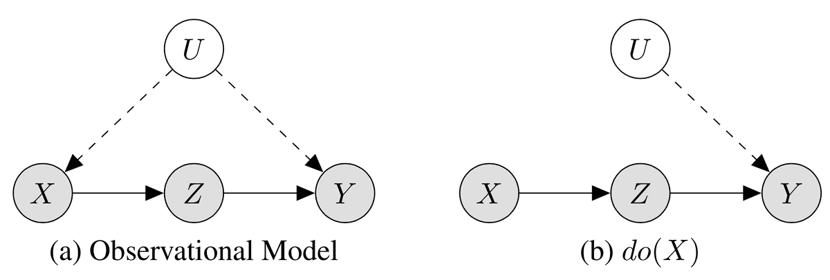
Example: smoking and lung cancer. Let X indicate smoking, Y indicate tar buildup in the lungs, and Z indicate lung cancer. Suppose that these are observed, but we also hypothesize a hidden confounder U (perhaps genetic or societal factors):
- We are interested in the effect $p(y | do(x))$ . In the mutilated graph $G_{\overline{X}}$ on the right, we can write this conditional as $p(y | do(x)) = \sum_{z, u} p(y| z, u, do(x)) p(Z=z | do(x)) p(u)$ . Note that we need to keep the $do(x)$ conditioning, even where we could otherwise drop conditioning on $x$ , in order to indicate that we are still in the mutilated graph.
- By the backdoor criterion, we have $p(Z=z | do(x)) = p(Z=z | x)$ .
- By rule 3, we also have $p(y | z, u, do(x)) = p(y | z, u)$ .
- In order to get an estimate in terms of real-world quantities, we'd need to sum out the $u$ . To do this, we need: $\sum_u p(y | z, u) p(u) = \sum_{u, x} p(y | z, u, x) p(u, x) p(z | x) / p(z | x) = \sum_{u, x} p(y | z, u, x) p(u, x, z) / p(z | x) = \sum_{u, x} p(y | z, u, x) p(u, x | z) p(z) / p(z | x) = \sum_{x} p(y | z, x) p(x | z) p(z) p(x)/ p(z , x) = \sum_{x} p(y | z, x) p(x)$ . (this is not the shortest derivation, but I did make it work).
- Therefore we have $p(y | do(x)) = \sum_z p(z | x) \sum_{x'} p(y| z, x') p(x')$ . This formula turns out to be known as the front-door adjustment
- TODO finish this: sources Introduction to Causal Calculus (ubc.ca) Lies, Damned Lies, and Causal Inference | Keyon Vafa

do-calculus

Links to this note

infinitesimal

causal inference

counterfactual

do-calculus

potential outcomes

Meta